
Everybody has likely already realized that there's essentially no facts that we can not get. we are able to get records about our website through the use of free equipment, however we additionally spend lots of money on paid tools to get even more. examining the competition is barely as handy, competitive intelligence tools are in every single place, we regularly use Compete or Hitwise. Opens web site Explorer is incredible for getting more data about our and opponents back-link profile. No rely what counsel we are trying to get, we will, with the aid of spending fortunes or no funds. My favorite half is that almost each device has one average feature and that is the "Export" button. here is the most powerful function of all these equipment as a result of through exporting the facts into Excel and we will model it, filter it and mannequin it in any manner we want. Most of us use Excel on the regular foundation, we're widespread with the simple functions but Excel can do approach greater than that. In the following article i will try to current essentially the most usual statistical options and the better part it is that we do not need to memorize advanced statistical equations, it be every little thing developed into Excel!
records is all about amassing, inspecting and decoding facts. It comes very convenient when resolution making faces uncertainty. through the use of information, we can overcome these cases and generate actionable analysis.
records is divided into two foremost branches, descriptive and inferential.
Descriptive data are used if you happen to understand all of the values in the dataset. for example, you're taking a survey of 1000 people asking in the event that they like oranges, with two selections (sure and No). You compile the results and also you find out that 900 answered yes, and a hundred answered No. You discover the percentage ninety% is sure 10 is not any. pretty fundamental appropriate?
however what occurs once we can not look at all of the facts?
if you understand most effective a part of your records than you should use inferential statistics. Inferential data is used in the event you know handiest a sample (a small half) out of your information and you make guesses in regards to the total inhabitants (records).
Let's accept as true with you are looking to calculate the email open expense for the last 24 months, however you've got facts best from the last six months. in this case, assuming that from 1000 emails you had 200 people opening the e-mail, which resulted in 800 emails that didn't convert. This equates to twenty% open expense and eighty% who didn't open. This information is true for the closing six months, but it could now not be actual for twenty-four months. Inferential information helps us have in mind how close we are to the whole inhabitants and the way assured we're during this assumption.
The open fee for the pattern can be 20% nonetheless it might also vary a bit. for this reason, let's agree with +- three% during this case the latitude is from 17% to 23%. This sounds relatively good however how assured are we in these facts? on the other hand, how many of a random sample taken from the entire inhabitants (data set) will fall in the latitude of 17%-23%?
In statistics, the 95% self assurance degree is regarded to be authentic statistics. This potential ninety five% of the sample statistics we take from the complete population will produce an open expense of 17-23%, the other 5% should be either above 23% or below 17%. but we're 95% bound that the open cost is 20% +- three%
The time period statistics stands for any cost that describes an object or an experience corresponding to visitors, surveys, emails.
The time period records set has two add-ons, observation unit, which is as an example visitors and the variables that can signify the demographic features of your guests corresponding to age, income or training degree. population refers to every member of your neighborhood, or in internet analytics all the friends. Let's assume 10,000 friends.
A pattern is only a part of your population, in accordance with a date latitude, visitors who transformed, etc. but in statistics essentially the most helpful sample is considered a random sample.
The information distribution is given by way of the frequency with which the values within the records set happen. with the aid of plotting the frequencies on a chart, with the range of the values on the horizontal axis and the frequencies on the vertical axis, we acquire the distribution curve. probably the most usual distribution is the regular distribution or the bell-formed curve.
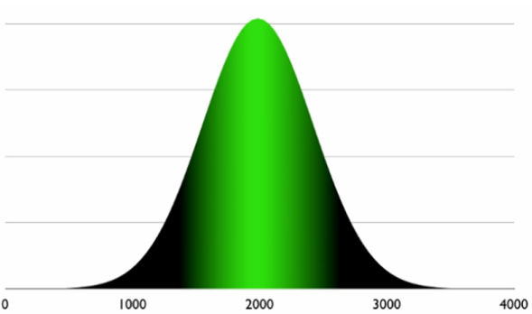
an easy solution to take into account this is with the aid of when you consider that the number of company a website has. for example the number of visits are on regular of 2000/day however happens to have greater visits equivalent to 3000 or less one thousand.
here, likelihood conception turns out to be useful.
probability stands for the chance of an event happening similar to having 3,000 friends/day and is expressed in percentages.
essentially the most common illustration of likelihood that likely everybody knows is the coin flip. A coin has two faces, head and tail, what's the chance when flipping a coin to have head? well there are two chances so a hundred%/2=50%.
adequate with theories and let's get a bit bit more purposeful.
Excel is a good tool that can help us with facts, or not it's not the top of the line but all of us comprehend how to use it so let's dive right into it.
First, deploy the evaluation ToolPack.Open Excel, Go to options -> Add-ins->on the bottom we are able to locate
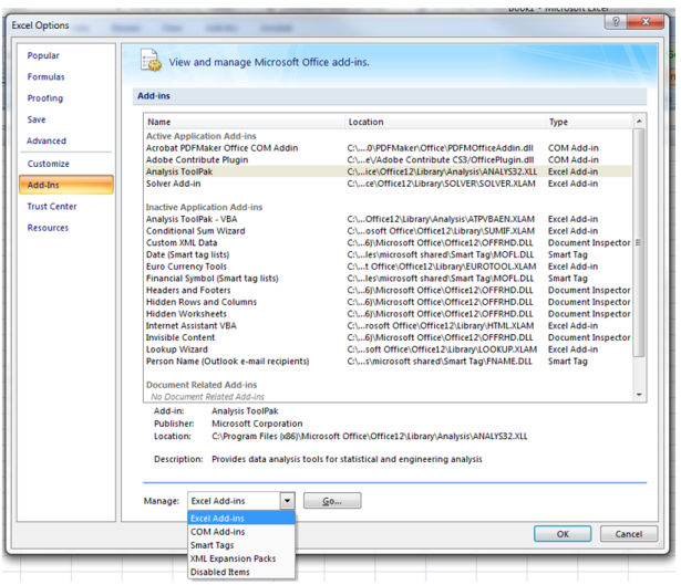
Hit Go ->opt for analysis ToolPack->and click adequate.
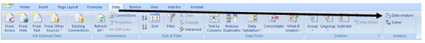
Now beneath the data tab we can discover information evaluation.
The statistics analysis device can provide you supper fancy statistical counsel however first let's start with some thing less difficult.
imply, Median, and Mode
imply is the statistical which means of normal, for instance the mean or standard of 4,5,6 is 5 how we calculate in excel the suggest? =regular(number1,number2,etc)
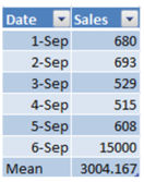
mean=usual(AC16:AC21)
with the aid of calculating the imply we understand how tons we offered on general. This assistance is helpful when there aren't any intense values (or outliers). Why? It seems like we bought on usual $3000 value of products, however in reality we have been fortunate that someone spent extra on September 6. however in fact we did pretty poorly right through the outdated six days, with a normal of only $618. apart from the extreme values from the imply can replicate a extra imperative performance fee.
The median is the observation headquartered in the middle of the facts set. for instance, the median of 224, 298, 304 is 298. with a purpose to calculate the imply for a big set of statistics we will use right here components =MEDIAN(224,298,304)
When is the median positive? well, the median is effective if in case you have a skewed distribution, as an example you're promoting goodies for $three up to $15 a bag but you have some very high priced candies for $100 a bag that no one in fact purchases on a daily basis. at the end of your month you need to make a report and you will see that you simply bought mainly low-cost goodies and only a few the $100. during this case calculating median is more a good option.
The easiest method to examine when to make use of the median vs. the mean is with the aid of making a histogram. if your histogram is skewed with an severe, you then understand that the most fulfilling approach to head is by calculating the median.

The mode is essentially the most ordinary cost, for instance the mode for: four,6,7,7,7,7,9,10 is 7
In Excel you can calculate the mode through the use of the =MODE(4,6,7,7,7,7,9,10) formula.
despite the fact this appears first-rate bear in mind that in Excel the lowest mode is regarded, or in different words, in case you should calculate the mode for here information set 2,2,2,four,5,6,7,7,7,eight,9 you can see that you've two modes, 2 and 7 but Excel will show you handiest the smallest price: 2.
When do we use the mode function? Calculating the mode is really useful only for total numbers corresponding to 1, 2 and 3. It is not positive for fractional numbers comparable to 1,744; 2.443; three,323, as the probability to have duplicated numbers, or a mode, is terribly small.
a pretty good instance of calculating the mode, or probably the most widely wide-spread number, can be probably on a survey.
Histograms
for example your blog currently acquired lots of of visitor posts, some of them are very respectable ones but some of them are just not that respectable. might be you need to see how many of your blog posts acquired 10 back-links, 20, 30 etc, or maybe you are interested in social shares akin to tweets or likes, however why not just with ease visits.
here we are able to categorize them into groups by using a visual representation referred to as histograms. during this illustration i will be able to use visits/articles as an easy example. the style I setup my Google Analytics account is as follows. I have a profile that tracks best my blog, nothing else. in case you don't have such profile setup yet, then that you may create a section on the fly.
How are you doing this? relatively elementary:
Now go to export->CSV
Open the excel spread sheet and delete the entire columns other than touchdown page and Visits. Now create the tiers (also called boxes) that you just wish to be categorized into. for instance we need to see how many articles generated a hundred visits, 300, 500 and so forth.
obtained to facts -> records analysis->Histograms->ok

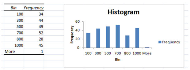
Now you have got a nice histogram that shows you the variety of articles categorized by visits. To make it less demanding to understand this histogram, click on any telephone from the Bin and Frequency table and kind the frequency with the aid of low to high.
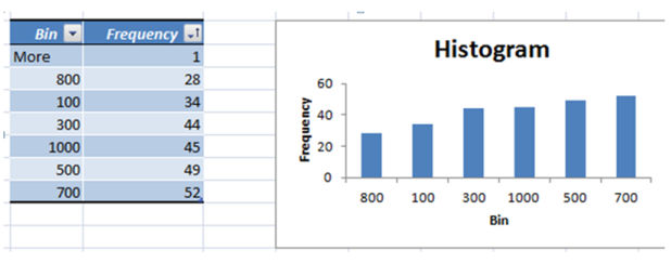
inspecting now the records is even more straightforward. Now go returned and sort all of the articles with much less or equal to one hundred visits (talk over with drop down->number filters->Between...0-one hundred->ok) within the remaining month and update them, or promote them.
Visits via supply
How useful this file is for you?
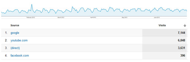
it be pretty respectable but not magnificent. we can see united statesand downs but...how a whole lot did YouTube make a contribution in February to the entire visits? that you could drill down however it's added work, and it is very uncomfortable when the query arrives on a cellphone name with a shopper. To get probably the most out of your graphs, create positive self-descriptive reports.
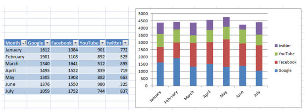
The file above is so a lot more straightforward to remember. It takes greater time to create it nonetheless it's more actionable.
What we are able to see is that in may, facebook had a bigger quantity of contribution to the full than in frequent. How come? likely the may advertising and marketing crusade turned into more helpful than in different months, resulting in a lot of traffic. Go returned and do it once again! If it was a working solution, then repeat it.
in case you believe that may additionally is only unintentionally larger than the rest of the months, then remember to create a Chi-rectangular verify to make sure that the increase in visits is not accidentally and it's statistically confirmed the effectiveness of your campaign.
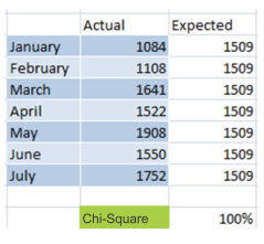
The exact column is the number of visits, the anticipated column is the mean(typical) of the "actual" column. The formulation of the Chi-rectangular test is =1-CHITEST(N10:N16,O10:O16) the place N10:N16 are the values from specific and O10:O16 the values from anticipated.
The effect of 100% is the self belief degree so you might have when because that the work invested in every month campaign affects the variety of company coming from fb.
When growing metrics, make them as effortless as viable to take into account, and principal to the enterprise model. all and sundry may still bear in mind your studies.
The video below explains pretty smartly a different illustration of Chi-square characteristic:http://www.youtube.com/watch?v=UPawNLQOv-8
moving normal and linear regression for forecasting
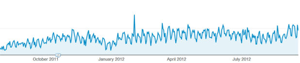
We regularly see graphs just like the one above. it may possibly represent revenue or visits, it would not actually count number, it's invariably going up and down. there's loads of noise within the records that we doubtless want to eliminate to generate a higher realizing.
The answer, moving commonplace! This technique is now and again used by way of merchants for forecasting, the stock prices are booming someday however in the 2nd they are hitting the flooring.
let's examine how we can use their basic ideas to make it work for us.
Step 1:Export to excel the number of visits/income for a very long time duration, akin to one or two years.
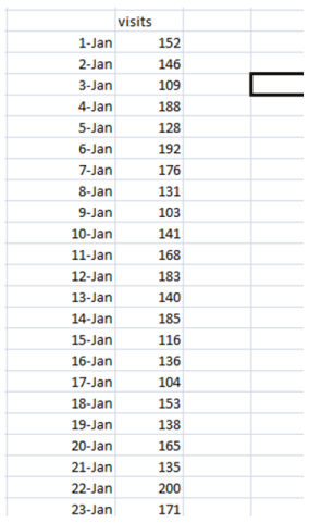
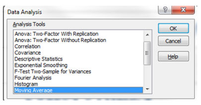
Step 2:Go to data-> information analysis -> moving general ->adequate
enter range might be the column with the number of visits
Interval might be the number of days on which the common is created. here you'll want to create one relocating ordinary with a far better number such as 30 and an extra one with a smaller quantity akin to 7.
Output latitude should be the column right subsequent to the visits column.
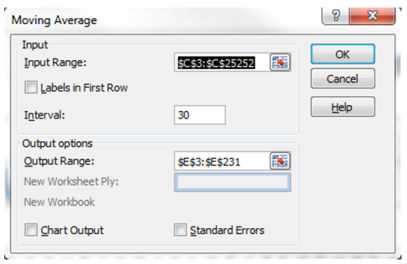
Repeat the steps for the interval of 7 days
very own option: I did not check the chart output and commonplace error field on purpose, i will create a graph later on.
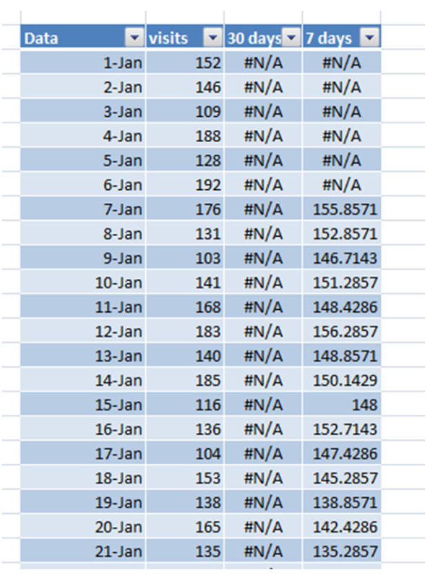
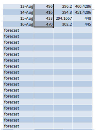
Your information now doubtless appears corresponding to this:
Now if you opt for the entire columns and create a line chart it will look like this:
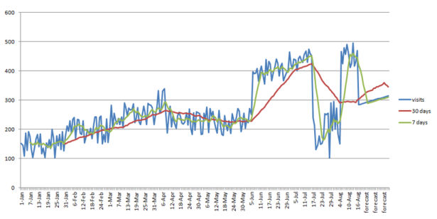
This illustration has much less noise, it's more straightforward to examine and it shows some developments, the green line cleans up a bit bit within the chart nevertheless it reacts to basically every essential adventure. The purple line as a substitute is greater strong and it indicates a true trend.
at the end of the line chart you can see that it says Forecast. it's forecasted facts in line with old tendencies.
In Excel there are two techniques for making a linear regression, the usage of the formula =FORECAST(x,known_y's, known_x's) the place "x" stands for the date you wish to forecast, "known_y's" are the visits column and "known_x's" are the date column. This approach isn't that advanced but there is an easier approach to do that.
with the aid of deciding on the entire visits column and dragging down the field tackle it will immediately forecast for the following dates.
note: be sure to opt for the whole records set with a purpose to generate an accurate data set.
there's a concept when evaluating a 7day moving usual and a 30day. As talked about above the 7day line reacts to almost every principal exchange whereas the 30day one requires greater time to change its course. customarily of thumb when the 7day relocating ordinary is intersecting the 30day moving commonplace then you could predict an incredible alternate so that it will final longer than a day or two. As which you could see above round April sixth the 7 day relocating usual is intersecting the 30 day one and the number of visits are taking place, round June 6th the traces are crossing once more and the tendencies are going upward. This technique is useful should you are dropping site visitors and you don't seem to be yet certain if it is simply the style or it is only an everyday fluctuation.
Trendline
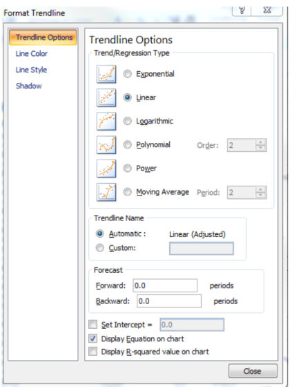
The identical outcomes will also be done through the use of the trend line function of excel: right click on the wiggling line -> choose: Add Trendline
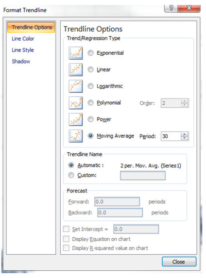
Now that you would be able to choose the Regression classification and you'll use the Forecast function as smartly. Trendlines are probably probably the most beneficial to discover if your traffic/income are going upward, downward or are with no trouble flat.
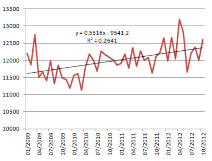
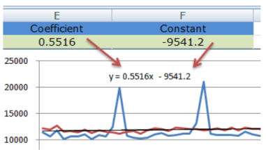
devoid of the linear function we can't confidently tell if we are doing better or not. with the aid of adding a linear trendline we can see that the slope is advantageous the trendline equation explains how our vogue is moving.y=0.5516x-9541.2
X represents the number of days. The coefficient to x, 0.5516, is a positive quantity. This capability that the trendline is going upward. In different words daily that passes by using we raise the variety of visitors with 0.5 as a vogue.
R^2 represents the level of accuracy of the mannequin. Our R^2 quantity is 0.26 which suggests that our mannequin explains 26% of the adaptations. effectively observed: we're 26% confident that every different day that passes with the aid of our number of guests increases with one new tourist.
Seasonal Forecasting
Christmas is coming soon and forecasting the iciness season can be beneficial chiefly when your expectations are high.
if you failed to get hit with the aid of Panda or Penguin and your earnings/company are following a seasonal vogue, then that you can forecast a pattern for income or visitors.
Seasonal forecasting is technique that permits us to estimate future values of an information set that follows a routine model. Seasonal datasets are in all places, an ice cream store could be very ecocnomic throughout the summer time season and a gift store can attain the highest earnings all through the winter vacation trips.
Forecasting data for close future may also be very a good option, specifically once we planning to make investments cash in advertising for these seasons.
here illustration is a primary model but this can be multiplied to a greater complicated one to suit your company model.
download the Excel forecasting instance
i will be able to spoil up the method into steps to be more straightforward to comply with. The gold standard way to put in force it for your business is by using downloading the Excel spreadsheet and following the steps:
with a purpose to calculate the index scroll down on the backside right of the spreadsheet and you'll find a desk referred to as Index. The index for Jan-2009 is calculated via dividing the revenue from Jan-2009 through the ordinary revenue of the complete year 2009.
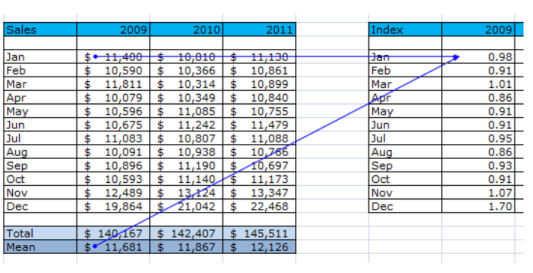
Repeat calculating the index for each month of every year.
In column S38 to S51 we calculated the commonplace index for every month
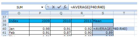
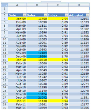
because our seasonality is every 12 month we copied the index capacity into column C over and over once again matching up every month. As which you can see January of 2009 has the equal index statistics as January 2010 and 2011
After growing the trendline and we displayed the Equation on the chart we trust the Coefficient the quantity which is elevated with the aid of X and the steady the number that's constantly has a negative sign.
We location the coefficient into phone E2 and the regular into mobile F2
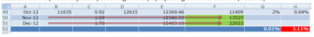
In my case cell F50 and F51 represents the forecasted statistics for Nov-2012 and Dec-2012. phone H52 represents the error margin.
through the use of this approach we will say that in December 2012 we're going to make $22,022 +- 3.eleven%. Now go to your boss and display him easy methods to predict the longer term.
normal deviation tells us how a great deal we deviate from the imply, in other phrases we are able to interpret it as a self assurance stage. for example in case you have monthly income, your each day income should be diverse each day. Then you could use the ordinary deviation to calculate how tons you deviate from the month-to-month standard.
There are two normal Deviation formulas in Excel that you should use.=stdev -when you've got sample data -> Avinash Kaushik explains in more details how sampling works http://www.kaushik.web/avinash/web-analytics-statistics-sampling-411/
or
=stdevp -if you have the total inhabitants, in different words you are examining each visitor. My very own option is =stdev just as a result of there are instances when the JS tracking code is not carried out.
let's have a look at how we can practice common Deviation in our everyday life
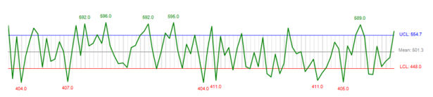
doubtless you see the wiggling graph in analytics every day but it surely is not very intuitive. by using general deviation in Excel you could easily visualize and take into account more desirable what's happening with your information. As you can see above, general every day visits have been 501 with a common deviation of fifty three, also essentially the most crucial, that you can see the place you passed the common so you can go lower back and take a look at which of your advertising efforts brought about that spike.
For the Excel document use right here link http://weblog.instantcognition.com/wp-content/uploads/2007/01/controllimits_final.xls
Correlation
Correlation is the tendency that one variable exchange is involving a further variable. a typical example in net analytics can also be the number of company and the number of sales. The more certified company you've got the extra sales you have. Dr Pete has a nice infographic explaining correlation vs. causation https://moz.com/weblog/correlation-vs-causation-mathographic
In Excel we use here formulation to investigate the correlation:=correl(x,y)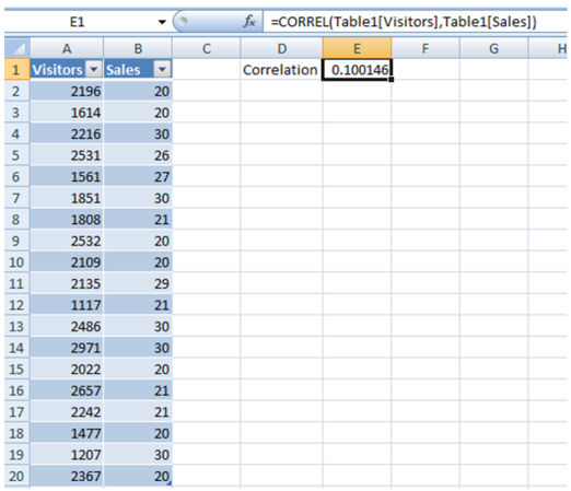
As you could see above we now have a correlation between Visits and revenue of 0.1. What does this suggest?
The conclusion in our case is that every day visits don’t have an effect on day by day earnings, which also means that the guests that you are attracting don't seem to be certified for conversion. You even have to agree with your business sense when making a call. but a correlation of 0.1 may also now not be neglected.
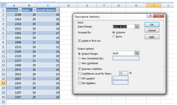
if you wish to correlate three or extra datasets that you can use the correlation function from the statistics evaluation device.
statistics->facts evaluation->Correlation
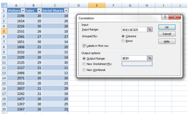
Your result will appear corresponding to this one: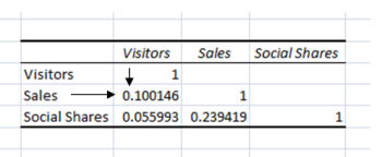
What we will see right here is that not one of the points correlate with each and every different:
Now you have decent figuring out of the mean, average deviations and many others. but calculating each and every statistical aspect can take a long time. The information evaluation device provides a brief abstract of essentially the most average features.
The result is fairly excellent:
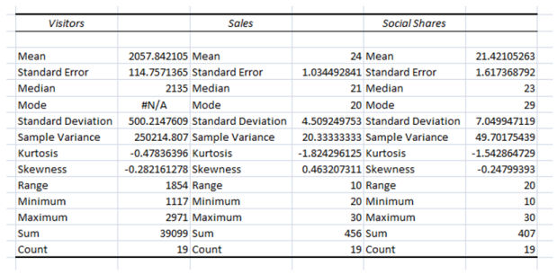
You already comprehend lots of the elements but what's new right here is Kurtosis and Skewness
Kurtosis explains how far peaked the curve is from the mean, in different words the bigger the kurtosis value is the bigger the top is on the sides, in our case the kurtosis is a very low number which means the values are spread out evenly
Skewness explains in case your records is negatively or positively skewed from a normal distribution. Now let me exhibit you extra visually what I suggest:
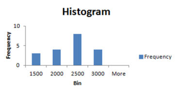
Skeweness: -0.28 (the distribution is more probably oriented towards the bigger values 2500 and 3000)Kurtosis: -0.forty seven (we've a really small height deviation from the center)
These are one of the vital options for you to use when analyzing information, the greatest problem behind data and Excel is the ability of making use of these strategies in various situations and never being restricted to visits or earnings. a very good example of distinct statistical procedures carried out together became realized through Tom Anthony in his submit about hyperlink Profile tool.
The examples above are only a small fraction of what can also be done with statistics and Excel. when you are the usage of different options that aid you're taking faster and improved selections i'd love to hear about them within the comment section.
No comments:
Post a Comment