Grab These Expert Excel Training Courses For Only $50

Microsoft Excel is hands-down one of today's most essential business tools, and understanding its ins and outs can take you far in practically any career. Want to make use of your free time and learn something that can pay off big down the road? Get the Excel training you need with The Premium A to Z Microsoft Excel Bundle, now discounted by over 90 percent today.

The Premium A to Z Microsoft Bundle is a web-based training resource geared towards people who are already working. The content is delivered entirely via the web so there are no actual classroom sessions to attend. You can literally log in at any time and train when you want to. And, as the content will be accessible for life, there’s no rush to complete it either. That makes it an ideal post-secondary training option as it fits with any existing work schedule, no matter how busy it is.

Aside from convenience, what really sets this program apart is the quality of instruction that’s offered. The 10-course collection features top-tier instructors including Alan Jarvis and Chris Dutton, both of whom are celebrated online instructors. They have, in fact, trained well over 200,000 people already, which is an amazing feat unto itself. And the training they’ve set up is so accessible that virtually anyone can understand it.

Even a complete beginner with no knowledge of spreadsheets, data analysis, or pivot tables can make sense of the courses here and become an expert. Just make your way through the training, and you'll have the know-how to save time with formulas, visualize valuable data insights in your spreadsheets, and even program your own Excel solutions using VBA.

When you compare this package to similar in-person programs, you’ll immediately notice the benefits. After all, with a flexible schedule, world-class training, and a no-pressure learning environment, students are in a better position to succeed. And, since The Premium A to Z Microsoft Excel Bundle is discounted by over 90 percent to just $49.99, it’ll be sure to fit even the tightest of budgets.

  The Premium A to Z Microsoft Excel Bundle Ft. Alan Jarvis & Chris Dutton - $49.99

See Deal

More from the PCWorld Shop

Prices are subject to change.

Note: When you purchase something after clicking links in our articles, we may earn a small commission. Read our affiliate link policy for more details.

Exam Prep for Bundle; Microsoft Excel 2013; Complete + ...

New Perspectives Microsoft Office 365 & Excel 2016 + SAM 365 & 2016 Assessments, Trainings, and Projects with 1 MindTap Reader Access Card: Intermediate

Microsoft ranges up word, Excel, and Outlook with more AI capabilities

Microsoft is adding a bunch of new capabilities to its workplace productiveness suite that are geared toward the usage of laptop gaining knowledge of to help americans get their work done extra efficaciously. Outlook, Excel, and word will all advantage, with new elements rolling out to a limited set of users within the coming months after which increasing to a broader set of americans in a while.

Outlook’s net customer will provide users with an interface if you want to immediately present them responses to questions layered inner emails, while Excel has a new characteristic that means charts and pivot tables. note will get a function in order to assist clients outline acronyms according to information shared within their corporation.

Above: An animation suggests Microsoft Excel’s new insight function.

graphic credit: Microsoft

The information is part of Microsoft’s ongoing push to enhance its productiveness suite for workers by way of offering them with clever features. all the aspects are designed to make it less demanding for individuals to get work executed speedy through decreasing the complexity of tasks interior office 365. They’re also designed to appeal to americans to Microsoft’s cloud productivity service, due to the fact all of these capabilities require processing on the enterprise’s servers.

The chance, besides the fact that children, is that whereas these capabilities sound first rate on paper, they can be just a little rough when the rubber meets the street. Microsoft is planning to roll out these facets to a small community of clients at the beginning, those who have expressed interest in checking out out the latest workplace elements, earlier than unleashing them on the rest of the area, in an attempt to make sure that they work the ultimate they can.

Microsoft isn’t on my own in pushing intelligent productivity capabilities, both: Google has spent time pushing its own computing device researching-based mostly elements interior G Suite, together with help for automatically producing charts and pivot tables. Inbox, Google’s experimental e-mail product that’s concentrated on productiveness, has a marquee wise Reply function that’s alleged to permit users to without delay reply to the content material of emails they obtain by clicking on considered one of three buttons.

The function that Microsoft offers in Outlook is designed to provide individuals more than only one response to an entire electronic mail, for greater advanced messages stuffed with a few questions. anywhere Outlook detects a question, it will supply users with a drop-down menu that comprises a series of immediately generated advised responses, in response to the content of the question.

moreover the question and answer function, Outlook is also dropping clutter, a characteristic that turned into speculated to take unimportant emails and shove them into a separate folder for later analyzing. That ability has now been rolled into the e-mail carrier’s concentrated Inbox function, which continues all of the messages a user receives of their inbox, but splits up how they’re displayed in line with even if Microsoft’s algorithm thinks they’re crucial.

Outlook for iOS clients will also get time to go away notifications, so that you can supply clients with suggestions about once they deserve to head out as a way to attain the subsequent experience on their calendar. It makes use of advice about traffic situations, strolling paths, and are living transit data to give clients an estimate of once they need to get relocating.

Excel will get a brand new Insights function that’s designed to immediately generate charts and pivot tables based on statistics clients enter to the carrier. The feature is meant to deliver shoppers with automated identification of particulars like outliers and tendencies within information that it’s been fed. actually drawing insights out of Excel may also be challenging for people who aren’t consultants at the use of the application, so this provider may additionally help democratize analysis for people who aren’t a part of the pivot table priesthood.

clients who are ill of getting misplaced in a sea of acronyms at work get a new feature in be aware. It tactics the entire files shared within a company the usage of the Microsoft Graph to drag definitions of usual abbreviations, so it’s less complicated for folks to grasp WTF a TPS report is. diverse corporations will get diverse definitions, depending on how americans use acronyms, on account that CYA can suggest different things at distinctive groups.

Must Have Spreadsheet Templates, Calculators, and Calendars

Let me tell you something. This is by far the best library of Excel resources we have found on the world wide web. 

Since 2003, Vertex42® has been creating professionally designed spreadsheet templates for business, personal, home, and educational use. We love Microsoft Excel®, but are also a leading provider of templates for OpenOffice.org and Google Sheets. Our collection of financial calculators include some of the most powerful and user-friendly debt reduction and money management tools you can find. 

We also provide a large selection of templates for Microsoft Word® such as resumes, letters, or a business plan template that includes financial statements in Excel.

Get Your Templates Now

creating a simple Joyplot in Excel – Tutorial

Over on Twitter, I got here across this fascinating chart, aptly titled – Joyplot. it is the type of chart that makes you all curious and awed. So I did what any Excel nerd would do. Recreated it in Excel of direction. This submit takes you via the method.

top time for activities and amusement #dataviz. About time for a joyplot; might do a write-up on them. #rstats code at https://t.co/Q2AgW068Wa pic.twitter.com/SVT6pkB2hB

— Henrik Lindberg (@hnrklndbrg) July 8, 2017

First let me share the final outcomes.

Joyplot in Excel – peak time of the day for activities and leisure

right here is the final overlapped area chart with just a little of formatting thrown in. it is an attractive close imitation of Henrik’s customary chart. click on it to amplify.

creating Joyplot in Excel – Tutorial

As that you may wager, the chart is a simply an overlapped area chart (ie each and every area sits behind another, in contrast to stacked enviornment chart where they are umm, neatly, stacked!)

Let’s delivery with a glance at facts. Henrik’s original statistics has 10,656 rows, every row containing recreation identify, time and p value – how a whole lot survey respondents enjoyed [@activity] at the moment.

here's a photo of first few rows.

Scrubbing and re-arranging the records

As you can see, whereas this structure is brilliant for storing, it is very tedious if we wish to make one chart with all sequence. So let’s scrub.

We need to determine if an endeavor may still be included or now not. i am using the equal standards as Henrik’s. Exclude actions with p value less than 0.003 or endeavor title “taking part in activities n.e.c. *”  (no longer in different places categorised)

To do this, we first pivot the information on pastime and max(p). Then filter this pivot two ways – max(p) >=0.003 and label no longer equal  enjoying sports n.e.c. * Tip: You may wish to allow dissimilar filters per field within the box settings of row labels.

we will emerge as with 28 actions.

Then add a helper column to common desk that looks up the pivot and tells if an undertaking should still be protected or no longer

Add two more columns to fashioned table to tell height time and modified time. this can support us in rearranging and sorting the facts. Modified time just strikes time by means of three hours (Henrik’s chart is plotted from 3AM to 3AM). At this stage our facts feels like this:

Now, pivot the facts once once again. This time,

exclude activities by using record filter on consist of? column.

set up top and endeavor in row labels enviornment, modified time in column labels enviornment and p in values enviornment.

organize the report in tabular structure, flip off sub-totals.

We get this:

Calculate normalized values by means of dividing every p price with maximum p value for that pastime. we are able to use a further latitude of 28×288 cells to do this. We get this:

The next 2 steps can also look puzzling. it will turn into clear once you appear at the charts.

outline an offset price. beginning with 0.5. which you can alternate this later. In a separate 28×288 phone range, calculate gaps by way of multiplying offset with place of an recreation. some thing like this:

Now, at last calculate activity + hole values by way of adding up respective cells in every of the 28×288 tiers. We get this:

At this stage, our statistics is a shape ready for visualizing.

creating and formatting overlapped enviornment chart

The chart creation process has 5 steps.

choose the 28×288 latitude of cells created in step 7 and insert an overlapped enviornment chart.

Now, reproduction the gaps latitude (created in step 6 above) and paste them on to enviornment chart as new collection (just ctrl+c your statistics and select the chart, press ctrl+v)

alter the order of sequence so that every pastime is sandwiched by accurately named hole sequence

Tip: adjusting fifty six series is painful with the chart select records > stream sequence up/down buttons. in its place, simply select the collection, analyze system bar. The series formulation has final parameter as order. alternate this number. it is handy to determine the number once you try a couple of.

exchange all gap collection fill colour to white. This straight creates the floating enviornment chart impact.

alternate the colorations of undertaking sequence. follow white / off-white border to those sequence. Your joyplot is equipped.

short overview of the chart advent manner:

Let’s assess the outcome of every these 5 steps with a smaller dataset so that you can see how everything matches collectively. right here is the records for this example:

Create an overlapped enviornment chart with activity+gaps information. We get this:

Add gaps as new series to chart. You get this:

movement the hole series in order that they sandwich undertaking sequence. Use Chart records > movement sequence up/down buttons or collection components

observe white color fill formatting for gap sequence. This creates floating area chart effect as below:

finally, format the chart by way of practice some colours and border formatting and so on.

So there you go. The final outcomes does appear happy.

alternate options to Joyplot

while joyplot is remarkable, it is not handy to make. happily, there are a number of less complicated alternatives that we can whip up in Excel as quickly as you've got both the pivot or normalized values.  under I even have shown two such examples. read about sparklines or conditional formatting heatmaps for more.

Joyplot choice – the usage of sparklines:

Tip: to get axis for your sparkline, simply class the instances separated by a single house. Then go to layout phone (ctrl+1) and set horizontal alignment to dispensed. Viola, Excel will fill the cell by adjusting areas.

Joyplot choice – Conditional Formatting Heatmap 

download Joyplot Workbook

click here to download Joyplot Excel workbook. determine the records scrubbing formulas, pivot and chart settings to learn how here is created.

if you're typical with R, then go thru Henrik’s R code. it's much shorter than the Excel gymnastics we did with circular pivot table referencing. That noted, one of the most statistics re-association may well be executed with same ease in vigour query too.

Your ideas on Joyplot?

The best step we missed in Excel implementation is relocating typical smoothing of the enviornment charts. It will also be without problems delivered as a step between 3 and four in statistics stage.

How do you like Joyplot? Would you create something like this for your company / very own records? Share your reports and ideas in the feedback section.

more joy for you…

Learn Advance Statistics Training in Excel

Solver: Excel 2013 Tutorial

Excel 2013 carries potent equipment to prevent hours of calculations. The Excel solver characteristic as an instance, can help you work out what most fulfilling stages of construction or income should be based on quite a lot of ambitions and constraints. This tutorial will exhibit you the way solver works and the way you can use it to investigate how many instruments to promote in distinctive branches of a firm.

if you're widely wide-spread with Excel and wish to take your capabilities to the next level, join gain knowledge of Microsoft Excel 2013 – advanced now and join over four thousand students who are gaining knowledge of to make use of Excel like a professional. This course presents over fifty two classes and 12 hours of video content material to train you how to take skills of advanced Excel services. you'll find out how to work with dates and times, how to calculate depreciation, the way to insert and layout tables and the way to work with Pivot tables and charts.

For this tutorial we can expect you're employed for a computer company that has branches in California, Texas and Ohio. The enterprise produces laptop’s that they promote at each and every of the distinctive branches at distinctive prices in line with the enviornment since the pc’s in California are just a little faster and for this reason individuals pay a bit of greater for the workstation than in Ohio, for example. We understand the inputs for every laptop and we also how many devices of enter we've. What we should determine is what number of workstation’s we should make in every area to maximise the business’s profit. If we manually calculated the figures, it could take hours to figure out the most profitable aggregate, but with Excel Solver, Excel does the give you the results you want.

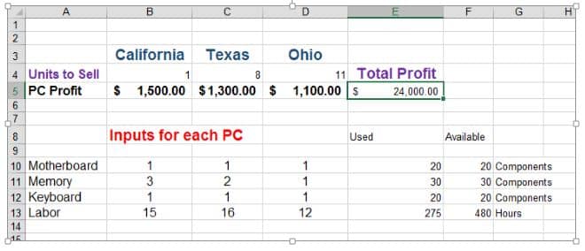
right here is the information we should begin with:

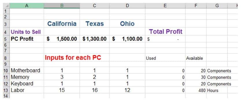
We comprehend the sales fee of the computing device’s in each and every enviornment – proven within the computing device income column. We also know what the inputs are for each enviornment – seen beneath the Inputs for every computing device. We also be aware of how many inputs we now have reachable.

Our objective is to maximise income so cellphone E5 might be our objective phone and it'll demonstrate us what profit we are able to make if we promote the top-rated variety of computers in every branch.

Our variables for this issue are the unit revenue for each enviornment. The income are represented by means of B4; C4 and D4. We want Excel to work out what the most reliable income for every department could be in line with the inputs we ought to maximize our profit.

The accessories we now have represent the constraints of the difficulty. we will’t make extra instruments than we have in inventory.

So we now have all of the accessories we need to get Excel to use the solver to work out the choicest mixture of earnings for each branch.

Add the formulas for the Cells

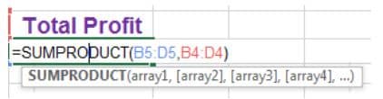
Add the formulation for the overall income:

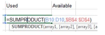
we will use the SUMPRODUCT formula to calculate the income. earnings is calculated via multiplying the units bought instances the unit expense for each area. we will use the equal SUMPRODUCT system to calculate what number of inputs are used for every classification of component:

Our worksheet now consists of the entire formulation we need to calculate the premiere level of revenue per department.

For training on the superior functions available in Excel, enroll in Microsoft Excel 2013 advanced online Excel practicing route now and be part of over twenty three thousand students who're studying to harness the power of the advanced elements and services in Excel. This course offers over 128 lectures and over 10 hours of content designed to take your Excel talents to the next stage. you will benefit a high-quality realizing of many of the powerful aspects attainable in Excel and after the direction you'll think at ease about the use of Excel in any commercial ambiance.

using Excel Solver

click on the statistics tab after which click on solver. Solver opens a brand new window to can help you add your constraints and aims: 

click on the “Set purpose” container after which opt for the income cell – this can set the aim because the maximum sales that Excel can calculate in response to the variables and constraints. we are able to go away the “To:” cost at Max due to the fact we need to achieve optimum earnings.

The variables for our calculation are the revenue per branch. What we try to work out is the superior combination of sales per department to maximize income so the variables are sales per enviornment. So choose cellphone B4:D4 because the variable latitude.

Now we need to add the constraints to our solver. The constraints involved during this illustration is the indisputable fact that we can not produce greater computer systems than we've components for and we also can’t produce a element of a computer – we should produce one complete computer at a time.

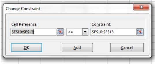
To enter the first constraint, we hence should say that the accessories used should now not be better than those we have on hand. So click “Add” so as to add a constraint. Then select E10:E13 – this could be the number of contraptions used to supply the pc’s and then opt for the “<=” and then select F10:F13. In different words we're telling Excel that the variety of devices used should be below or equal to the devices we've reachable. The constraint will look like this: 

Now we ought to add a constraint to make certain that Excel is aware of it can’t produce lower than one laptop. The constraint will therefore be unit income should be better than or equal to at least one. 

Now that we've all of the add-ons, click on clear up.

The reply looks as follows: 

it might have taken hours and many calculations to work out the combination, however Excel’s solver 2013 has grew to become the problem into an answer in no time in any respect.

become an Excel master. try Microsoft Excel 2013 rookies/Intermediate practicing and go from zero to Excel hero. This route presents over 58 lectures and 14 hours of content material designed to take you from beginner degree in Excel to Excel grasp. The course will introduce you to the fundamentals of Excel and then build for your talents unless you're capable of grasp superior Excel topics like working with Pivot charts, analyzing facts and fiscal evaluation.

5 easy methods to Double verify Your Excel formulation.

whats up Excellers. i am excited to share with you some more method enjoyable, and in specific a guidelines to double check your Excel formulation are on aspect!.

Let’s face it, formulation are unbelievable, however they could can additionally trigger massive headaches even with a tiny mistake, Excel will go ahead and do what you tell it to, so you ought to be certain your are giving it the appropriate guidance. here is an easy checklist to double check your Excel formula work.

1. Are You blended Up?…..

it is fantastically effortless to get all combined up principally if you have a tonne of formulation going on in your worksheet. from time to time it is not so effortless to identify blunders with mix ups.

This method =D2-D3 appears at lot like =D3-D2. Take a few minutes to ensure there aren't any small discrepancies like this one.

2. Roughly know What You answer should still Be…..

if you're in a position to, then take a stab at a ballpark effect in your formulation. I do this when checking my formulas, as an instance the calculation maybe the percent change between two sales figures as in my example beneath. i know that it should be a negative number, and round about a quarter?. This gives ball park evaluation to assist me spot and evident concerns with my formulation. this is a really simple method to check formulas, like in my example understanding it's a poor number, but the rest greater specific, it’s not so helpful. you can at all times substitute some standard numbers in the system to make it less demanding to determine what the reply may still be.

 three. check The Order Of Precedents or Operations.

What the heck does that suggest?, smartly, it is lower back to some fundamental mathematics classification…. but this relates to the order during which Excel calculates.

It’s crucial to keep in mind that for those who create a components with several operators, Excel evaluates and performs the calculation in a selected order. for instance, Excel at all times performs multiplication earlier than addition. This order is known as the order of operator precedence. you can force Excel to override the constructed-in operator priority through the use of parentheses to specify which operation to consider first.

Then order of calculations may also be with ease remembered through the acronym BEDMAS

Brackets

Exponents

Division

Multiplication

Addition

Subtraction

here is an illustration. right here components produces 11 as a result of Excel calculates multiplication earlier than addition. The system multiplies 2 via 3 and then provides 5 to the result.

=5+2*three

In distinction, in case you use parentheses to alternate the syntax, Excel adds 5 and 2 collectively and then multiplies the result by means of three to provide 21.

=(5+2)*three

See how this changes issues?…. in case you need to see greater instance of this in action take a look at my blog submit method Friday – How Excel Calculates – The Order Of Excel Calculations.

4. change Your View To demonstrate formulas…

a very quick method to check formulas is to make use of the reveal formula function. This allows you to see the entire formulas on your worksheet on the equal time. There are a couple of easy methods to try this.

Hit the CTRL+` shortcut (the grave accent)

formulas Tab – system Auditing – reveal formulation

which you could now see the formulation.

5. be certain All formula Arguments Are Accounted For…

if you're the use of a feature in Excel then it could actually have distinctive arguments that are required. If here's the case then make sure they are all accounted for. As you begin to category the feature, Excel will reveal the dialog field to e-book you during the ingredients of the method.

formulas get simpler with follow and even more observe. in case your formulation returns an error, or isn't giving an expected influence, then work via some troubleshooting within the steps above. The error is always evident when you look for it after which easily fastened.

Don’t neglect to check in to the Excel at Excel newsletter for 3 free Excel counsel the primary Wednesday of the month. just click on the sign up form to the right or use the link under.

Advanced Statistics Training in EXCEL

Convert incoming XML to Excel Sheet

Currently most of our clients got here with a requirement to create an excel file as an output of an xml. state of affairs was Proxy-SAP PI 7.31 (Java Stack)-Third celebration – output as Excel Sheet. First PoC of this requirement was to create a goal file by simply giving output.xls and see what fields populated. As anticipated output get populated as xml.

To populate goal file as Excel file we need to do transformation somewhere between the XML got and target file generation. we have 2 options –

Transformation at the time of Mapping

Write Adapter Module in Java

on the time of mapping we are able to achieve excel output via XSLT mapping. For this answer we deserve to convert incoming XML file to MS Excel XML structure.

For the conversion of XML to MS Excel XML format we need to use under code in xslt.

<?mso-application progid="Excel.Sheet"?><xsl:stylesheet version="1.0"xmlns:html="http://www.w3.org/TR/REC-html40" xmlns:xsl="http://www.w3.org/1999/XSL/radically change" xmlns="urn:schemas-microsoft-com:office:spreadsheet" xmlns:o="urn:schemas-microsoft-com:office:workplace" xmlns:x="urn:schemas-microsoft-com:workplace:excel" xmlns:ss="urn:schemas-microsoft-com:workplace:spreadsheet">

explanation of this scenario can be found below.

Convert incoming XML to Excel or Excel XML – part 1 – XSLT means

second option is to write down an adapter module to transform incoming XML to CSV and then to Excel Sheet.

Pre-Requisite and Assumptions of the building:

1. Apache POI open average for excel Conversion

2. SAP PI specific development libraries

  com.sap.aii.af.cpa.svc.api.jar

  com.sap.aii.af.lib.mod.jar

  com.sap.aii.af.ms.ifc_api.jar

  com.sap.aii.af.svc_api.jar

complete clarification of this state of affairs can be discovered below.

LEARN MORE



Links and related books

Excel 2007 VBA Macro Programming

Microsoft Excel VBA Programming for the Absolute Beginner

Learn Advance Statistics Training in Excel

Primary Excel Parser

A simple excel parser that parses every row to an associative array.

When to use this?

Your excel file has the header on the first row, and records on the leisure rows.

You want to map the header titles to database keys.

You wish to map the information values to database enums.

example

You need to parse an excel file with this format.

identify Age Gender mobilephone 1 cell 2 invoice 18 Male 222-222-2222 777-777-7777 Peter 25 Male 222-333-4444 555-666-7777 Monica 31 female 666-666-6666 555-555-5555

and you wish to map the header titles to database desk fields, and map genders to 'm' or 'f'.

$parser = new Jhesyong\Excel\Parser; // Map 'identify' to 'name', 'Age' to 'age', and 'Gender' to 'gender'. $parser->addHeader('identify', 'name'); $parser->addHeader('Age', 'age'); // Map the values: 'm' is for 'Male', and 'f' is for 'female' $parser->addHeader('Gender', 'gender')->withOptions(['m' => 'Male', 'f' => 'Female']); // you can use a daily expression and move a callback to map numerous header titles. // in this case, 'cell 1' may be mapped to 'phone_1' $parser->addHeader('/^cell \d+$/', characteristic($title) return str_replace(' ', '_', strtolower($title)); ); // Load the file and start to parse. flow a callback feature // and it will be called for each row. $parser->loadFile('filename.xlsx')->parse(characteristic($information) // information could be an associative array. var_dump($statistics); ); FAQ I actually have distinctive titles of the equal textual content, but I are looking to map them to distinct database table fields.

you can add headers with the same title however distinctive box names within the desired order.

// the first 'phone' should be mapped to 'phone_1', // and the 2d 'cell' can be mapped to 'phone_2' $parser->addHeader('phone', 'phone_1'); $parser->addHeader('phone', 'phone_2'); I just want to use the title as the container name

that you would be able to omit the 2nd argument.

// 'cellphone' can be mapped to 'mobile' $parser->addHeader('phone'); I need to pre-define the header mapping and the alternate options.

that you would be able to prolong the Parser and write your rules in the constructor.

TRY IT OUT

Links and related books

PHP: MySQL in 8 Hours, For Beginners, Learn PHP MySQL Fast! Hands-On Projects! Learn PHP MySQL Programming Language with Hands-On Projects in Easy Steps, A Beginner's Guide. Start Coding Today!


Programming 5:C Programming Success in a Day & Excel Shortcuts (C Programming, C++programming, C++ programming language, Excel, Javascript, Programming, Microsoft Excel, Python, Java, PHP)


Java Artificial Intelligence: Made Easy, w/ Java Programming; Learn to Create your * Problem Solving * Algorithms! TODAY! w/ Machine Learning & Data ... engineering, r programming, iOS development)

Excel to Html

Description

Finally a good program that will help you to import data in the web. Stop to write the data in the tables html, you just have to change the data inside the file Excel and this application read your excel and create the table html responsive with sorting..

Table Responsive

Contact Form

Google Maps

Features

• 100% Responsive
• Table Sorting
• Pagination Table
• Search for column
• Ajax Contact Form
• Single Table with 2 design
• Multi Table
• Google Maps
• Browser Compatibility
• Google fonts included

INSTALL

Generating Personalized Letters Using CSV Data From Google Spreadsheets

Google Spreadsheets are great for collaborative number crunching. Much like Microsoft Excel, Google Spreadsheets allow you to produce financial models, analyze numerical data, keep track of accounts, etc. But what if you want to produce and deliver documents of a different nature, like letters to various recipients, based on the data contained in a Google Spreadsheet? Instead of going through each row of the spreadsheet one at a time and plugging data into a document template manually, you can use WebMerge to pull data from the spreadsheet and automatically fill in a template document, perhaps, to be delivered in PDF form to certain recipients!

"How can I do this?" you might ask. Don't worry! We’ll walk through the process in the tutorial below.

First, we’ll need to have a document ready for merging on WebMerge. In this example, let’s say we want to send students a report card based on data we have in a Google Spreadsheet. In the spreadsheet we have the students’ names, their email addresses, and their GPAs.

We first go to WebMerge and upload or create a new document in the Document Builder. The document we are about to upload or create is the document that will be automatically populated with the data from our Google Spreadsheet. Our merge document might look something like the following. The following is an example of a cover letter with merge-fields for the students’ names and the students’ GPAs. The merge fields will get populated with the data in our spreadsheet.



After we have our document template on WebMerge, we want to: make sure our configuration settings are how we want them, test our document, and set up delivery.  Notice that in the delivery setup, we specify an <<other>> merge field. We didn’t create a merge field for the students’ email addresses, but we want to use the email address column in our spreadsheet to specify our email recipients.



The above shows that we want to send the document to recipients according to a merge field that wasn’t in our document and has as yet to be specified. We want to send emails to the addresses in the email address column of our spreadsheet, so we specify that we want to create a new merge field called Email_Address and use it as a placeholder for the email addresses in our spreadsheet. In the next step we will match this placeholder as well as the placeholders in our document with the data we get from a CSV version of our spreadsheet.

Now that we have made our document template and have saved our delivery method, we need to pull the information from our Google Spreadsheet. The easiest way to do this is to simply download the spreadsheet as a CSV file.



Once we have downloaded our data as a CSV file, we can upload that to WebMerge.



Upload the data, then in our final two steps we map the merge fields to the columns of our spreadsheet and send our newly created documents off to our recipients.



Click Merge the Data!



Congrats! You just merged your Google Spreadsheet data with a document template and sent it to all the relevant recipients.



Want to do more with WebMerge? Check out all the ways you can streamline your documentation process today!

Suggested Posts: 

Take Your Mail Merge Online

New: Merge Excel Spreadsheets on the Fly

10 signals Your advertising team Have Outgrown Excel Planning

Get Started Now!